Deep Reinforcement Learning: From SARSA to DDPG and beyond

It was only a couple of years ago that DeepMind’s AlphaGo algorithm beat Go world champion Lee Sedol. This spectacular feat was made possible with the help of Reinforcement Learning but unquestionably did not come overnight. The research for this ambitious project started in the early 2000s. And the field in itself has progressed a lot since then. This article aims to cover a part of the transformation towards modern approaches.

Basics

Before we begin, we have to narrow down the meaning of Reinforcement Learning: The goal of Reinforcement Learning is to act as good as possible. This definition is a simplified version of

The goal is to find a policy that maximizes the expected return.

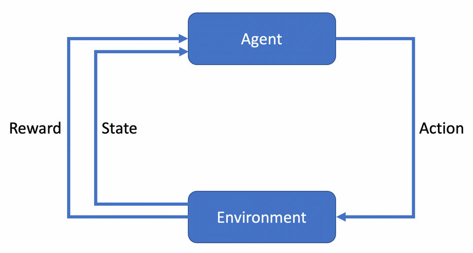
For this to happen, we have several components that work together, as can be seen in this image:

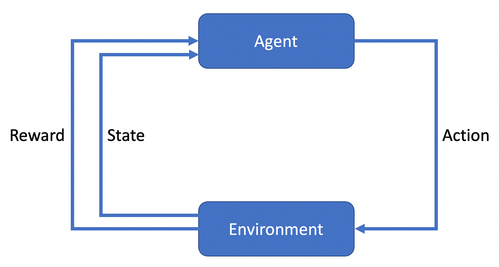
The agent interacts with an environment, which changes its state and yields a reward for the action. Then, another round begins. Mathematically, this cycle is based on the Markov Decision Process (MDP). Such an MDP consists of five components: S, A, R, P, and p₀.

S is the state space, which holds all possible states s that the environment can be in. For example, if we were to model a car, it might have the following states: moving forward, moving backwards, turning, braking, and so on.

The second component, A, is the action space, which defines all actions a that the agent can perform. For the car setting, this could be turning the wheel, accelerating, braking. Such actions lead to new states.

The third component, R, is the reward function. This function is responsible for rewarding an agent based on its action and the resulting state. For example, if the car successfully stopped at a traffic light, the agent would get a positive reward. However, had it not stopped, the agent would have gotten a negative reward.

The fourth component, P, is the transition probability function. Often, it can be that an action is not guaranteed to lead to the desired state. Therefore, this property is modelled as a probability function. For example, it might say: “With a chance of 90%, we land in the desired state, but with 10%, something different might happen.”

Lastly, we have p₀, which is the set of starting states. Every time that an agent is trained, it begins in one of these states.

Now that we have covered the ingredients of an RL setting, how can we teach the agent to learn the desired behaviour? This is done with the help of a policy, π, which I briefly touched upon before. Formally, a policy maps from the state space S to the probability of all possible actions. Sounds complicated? Consider this: You stand at the roadside and want to cross the roads. This situation is your starting state. A policy would now list all possible actions: Looking left, looking right, running straight forward, waiting, and so on. All these choices have a probability of being selected. For example, you might choose to look left with a 20% chance, and with a 50% chance, you might choose running.

As the agent is trained, it optimizes the policy. In the beginning, π might often select running across the streets. However, as the agent is repeatedly hit by cars, he gets many negative rewards, which he does not want. Over time, the agent learns to act better, leading to more and more positive rewards. Ultimately, this will lead to finding a policy that maximizes the total reward.

But, how do we know if the state that we are in is any good? And for the actions we can take, we might ask: How do we know if they are any good? This evaluation is achieved with the help of value functions. We have two of them, one for the states and one for actions.

The first function is called the state-value function and is abbreviated as V. For every state, it “knows” how good this state is. The state’s goodness is determined by the reward we expect to get when starting in this state. For example, the pole position in racing is more likely to win the race; this driver receives a positive reward. This fact influences the value of the pole position: As more and more people start here and win the game, the number of positive rewards that followed from this state increases. In turn, the value of the pole position increases.

The second function is the action-value function and is abbreviated as Q. For all actions that we can in a given state, it “knows” how good they are. This knowledge is gained similar to above: Actions that lead to a good reward have a higher value than actions that lead to negative rewards.

SARSA

Now that we have covered the basics, we can examine a classic RL algorithm called SARSA [1]. The name is an abbreviation for State Action Reward State Action, which neatly captures the functioning.

First, we start in a state (S), take action (A), and get rewarded (R). Now we are in the successor state(S) and choose another action (A). We do this to update our Q-function. As mentioned previously, the value of an action is the total reward that we expect when we start in a state and select this action. The same property holds for the next state, the next-next state, and for the next-next-next state. We can express this with the update rule of our action-value function:

Q(s,a) ← Q(s, a) + α(r + γ Q(s’, a’) — Q(s, a))

What does it say? The new value for our state-action pair is the old value plus, and this is the part in the brackets, the difference to what we get by going from here: r + γ Q(s’, a’). So over time, our Q-function gets closer to the reward that we get, which is modelled by this update rule.

Now that we have the Q-function (or Q values as they are sometimes called), what can we do with it? First, these values are stored in a table. Every time our policy has to select an action, it checks in which state it is and then looks at all possible actions:

From all these actions, the one with the highest value is chosen. This action leads to a new state, where once again, the best-valued action is chosen. During training, the Q-values are updated following the previously introduced update rule. Once it has finished, we have found a suitably good policy and are ready to use the agent in our environment.

But there is at least one point where we can improve the algorithm. That is where Q-Learning comes into play.

Q-Learning

The Q-Learning algorithm [2,3] can be summarized as off-policy SARSA. To explain this, let’s take a second look at SARSA’s update rule:

Q(s,a) ← Q(s, a) + α(r + γ Q(s’, a’) — Q(s, a))

Our policy π selects an initial action, which is the Q(s, a) part. Then, we use the same policy to select the subsequent action, which is the part that says Q(s’, a’). The process of using the same policy to determine both actions is denoted by the on-policy keyword. The agent learns the Q-value based on the action chosen by the policy currently used.

In contrast, in off-policy algorithms, we have more than one policy. This can be seen in Q-learning’s update rule:

Q(s,a) ← Q(s, a) + α(r + γ maxₐ’ (s’, a’) — Q(s, a))

The crucial difference is selecting the best successor action, which is not done by following the policy. Instead, we always select the action with the highest Q-value. This selection process can be understood as another policy used to determine subsequent actions. The benefit is that we can follow a different policy to select successor actions. This might not seem like a big deal, but in Q-learning, we use this fact always to choose an optimal subsequent action.

Further, it allows us to incorporate additional influences easily. For example, think about a second agent we might have. This agent has a unique feature, and we want our primary agent to learn it, too. We take the secondary agent’s policy and use it whenever we select a new subsequent action.

So far, we did not require any neural networks. But tabular methods do not scale well for large state and action spaces: First, their memory consumption is vast. Secondly, we might not even visit all states or actions during training, so some entries would be left uninitialized. Third, lookup times are prohibitive. However, as a first measure, we can use neural networks to replace the Q-tables.

Deep Q-Learning

Neural networks have been shown to generalize well. We can use their ability to learn features from data for Reinforcement Learning as well. In Deep Reinforcement Learning, we approximate our functions, such as Q, with neural networks [4]. To highlight this modification, the Q or V functions are often marked with θ: Q_θ and V_θ. There are methods beyond neural networks, but these are not the scope of this article.

In default Q-learning, the update rule helps us find optimal Q-values. Optimal means that they lead to the highest rewards; we can use them to select the optimal action (the one with the highest Q-value in a given state). And, by using neural networks, we directly approximate this optimal Q or V function. We learn from a small amount of training data and can then generalize to new situations.

In the Deep Q-learning algorithm, we use two techniques called experience replay and target networks.

The first modification stores old transitions (which are the moves from one state to the next by choosing an action) in a replay buffer. During training, we sample from this buffer. This technique increases efficiency and makes the data distribution more stationary. How is that? Now, think about what would happen if we had a couple of actions, and in each training step, we’d select a different one. We would always jump between the possibilities. With a replay buffer, we can detect trends in the distribution, making the selection of actions more stationary.

The second modification, target networks, is used when computing our targets. Generally, our target is to maximize the expected reward. The problem is, how do we know if our reward is not already the best possible one? The target networks help us solve this question. We use a network from an older update step and consider its Q-values as the target. This might sound difficult, thus let’s have a look at the update rule with target networks:

Q_θ(s, a) ← Q_θ(s, a) + α((r + γ maxₐ’ Qₜₐᵣ(s’, a’)) — Q_θ(s, a))

The difference is in the computation of the update goal. By minimizing the difference between our current value, Q_θ(s, a) and Qₜₐᵣ(s’, a’), we approach the target, abbreviated here as “tar”. And this target is the value of the target network.

Now, if we would not use such a target network but the current network Q_θ only, our target would constantly change: With every update of the network’s parameter, we’d get different Q-values. That’s why we use older networks (meaning from a few update steps before our current network) that serve as a fixed target. Its parameters are updated more slowly, making the target more stationary. In the end, we reduce the risk that our main network might end up chasing its own tail.

Put differently, think about a running competition. Every time you get close to the finish line, it moves back. This way, you never know how close you are to reaching the goal.

The two presented modifications, using a replay buffer and target networks, were used to help RL agents play Atari games, sometimes even at super-human level [5].

Deep deterministic policy gradient

So far, we have only considered discrete action spaces. In discrete action spaces, we have a fixed number of actions with only a single level of granularity. In contrast, think about an angle between a door and the wall. If we only have, say, two positions it can take, we have a discrete space. But we can place the door in any arbitrary position: Wide open, closed, 45 degrees ope, 30 degrees, 30.1 degrees, 30.01 degrees, and so on. That space is continuous and challenging to cover with both tabular methods and the Deep Q-learning approach.

The problem of continuous actions is the update step for the Q-function that we have so far:

Q_θ(s, a) ← Q_θ(s, a) + α((r + γ maxₐ’ Qₜₐᵣ(s’, a’)) — Q_θ(s, a))

The part where it says maxₐ’ Qₜₐᵣ(s’, a’) is the issue. In discrete action spaces, it’s easy to find the action that leads to the highest reward. However, in continuous action spaces with arbitrary fine-granular actions, this is very expensive, if not impossible.

A naive solution would be to discretize that space. But then, the challenge is how to discretize. However, we can skip this problem altogether and modify the Deep Q-learning algorithm to support continuous actions. This leads to the Deep Deterministic Policy Gradient (DDPG) algorithm [6,7], which essentially is Deep Q-learning for continuous actions. It also uses replay buffer and target networks but adapts the max-operation.

Instead of “manually” performing the search for the best state-action pair (the best Q-value), we introduce another neural network. This neural network learns to approximate the maximizer. Then, every time we query it with a state, it returns the best corresponding action — which is precisely what we need.

The new network, which replaces the maximizer, is then used in the calculation of the targets. Thus, the previous equation can be rewritten as

Q_θ(s, a) ← Q_θ(s, a) + α((r + γ Qₜₐᵣ(s’, μₜₐᵣ(s’))) — Q_θ(s,a))

As I’ve mentioned, we use the network, μₜₐᵣ, to determine the best action. As before, we use a slightly older version of the network, hence the “tar” part. Even though both μₜₐᵣ and Qₜₐᵣ are updated every step, they will never be updated to the most recent parameters. Instead, they usually keep 90% of their parameter values, and the remaining 10% come from the current network. This way, the target networks are neither too old nor too current.

The twin-delayed DDPG algorithm [8] introduces three modifications to improve the performance of the default version. First, TD3, as it is also abbreviated, learns two Q-functions and uses the smaller value to construct the targets. Further, the policy (responsible for selecting initial actions) is updated less frequently, and noise is added to smooth the Q-function.

Entropy-regularized Reinforcement Learning

A challenge for all algorithms is premature convergence. This undesired behaviour is a result of insufficient exploration. For example, if an agent has determined a good action sequence, he might focus on these particular actions. In this process, he fails to explore other states, which might have rewarded him even better. This phenomenon is also known as the exploration-vs-exploitation tradeoff: Exploration aims to explore the action and state space, while exploitation seeks to exploit the already explored area.

The entropy-regularized reinforcement learning approach is one way to tackle this challenge: We train the policy to maximize the tradeoff as mentioned above. To achieve this, we use a concept called entropy. Put simply, the entropy gives information about the “chaos” of a distribution. The higher the chaos (“the more uneven the distribution is”), the lower the entropy value is. Thus, a uniform probability, where all values have the same chance of being drawn, yields the maximum entropy value.

We utilize this fact by adding an entropy term to our value functions. Explaining them in detail exceeds the scope of this post, but the gist is the following: The additional term enforces the policy to maintain a balance between high reward (exploration) and choosing from a variety of actions (exploration).

In the Soft Actor-Critic algorithm [9, 10], this concept is, among others, used to train a robot to walk. While the robot was trained on flat terrain only, the resulting policy was robust enough to handle environments not seen during training.

Reinforcement Learning libraries

All of the algorithms above are already implemented in various python packages. The OpenAI Gym and Safety Gymframeworks provide code to build the environments that the agents are trained in. The researchers from DeepMind provide the Control Suite package, which is used for physics-based RL simulation.

To build algorithms, one can choose from a variety of options. The Stable Baselines 3 library is implemented in PyTorch and provides the tool to compare algorithms and create new ones, too. Similarly, the ACME library provides RL agents and building blocks and is flexible enough to do your own research. As the third alternative, one can consider Google’s Dopamine framework, which focuses on fast prototyping for speculative research. It supports JAX and TensorFlow.

Summary

The field of Reinforcement Learning has experienced a lot of critical ideas in the last decades. The foundation was set with the idea of learning functions that quantify the advantage of being in a particular situation. Researchers then proposed to use different policies to explore the environment efficiently. A significant step was made forward when the functions were learned with the help of Neural Networks, which introduced many new possibilities of algorithmic design. Over time, other ideas were included, such as gradually updating additional networks that serve as training targets. However, by no means is the development completed. There are still many challenges to be overcome, such as handling constraints, bridging the gap between the training and real-life environments, or explainability.

Literature

[1] Gavin Rummery and Mahesan Niranjan, On-line Q-learning using connectionist systems, 1994, Citeseer

[2] C.J.C.H. Watkins, Learning from delayed rewards, PhD thesis, 1989, King’s College Cambridge

[3] C.J.C.H. Watkins and Peter Dayan, Q-learning, 1992, Machine Learning 8

[4] Kurt Hornik, Approximation capabilities of multilayer feedforward networks, 1991, Neural Networks 4

[5] Mnih et al., Playing Atari with Deep Reinforcement Learning, 2013, arXiv

[6] Silver et al., Deterministic Policy Gradient Algorithms, 2014, International conference on machine learning

[7] Lillicrap et al., Continuous control with deep reinforcement learning, 2015, arXiv

[8] Stephen Dankwa and Wenfeng Zheng, Twin-delayed DDPG: A deep reinforcement learning technique to model a continuous movement of an intelligent robot agent, 2019, ACM

[9] Haarnoja et al., Soft actor-critic: Off-policy maximum entropy deep reinforcement learning with a stochastic actor, 2018, ICML

[10] Haarnoja et al., Soft actor-critic algorithms and applications, 2018, arXiv

[11] Haarnoja et al., Learning to walk via deep reinforcement learning, 2018, arXiv