Jul 10, 2021 21 min read Machine Learning

Natural Language Processing: From one-hot vectors to billion parameter models

Human language is ambiguous. Speaking (or writing), we convey the individual words, tone, humour, metaphors, and many more linguistic characteristics. For computers, such properties are hard to detect in the first place and even more challenging to understand in the second place. Several tasks have emerged to address these challenges:

Classification: This task aims to classify text into one or more of several predefined categories
Speech recognition and speech-to-text: These tasks deal with detecting speech in audio signals and transcribing it into textual form
Sentiment analysis: In this task, the sentiment of the text is determined
Natural language generation: This task deals with the generation of natural (that is, human) language

This list is by no means exhaustive; one could include Part-of-Speech tagging, (Named) Entity Recognition, and other tasks as well. However, the Natural Language Generation (NLG) field has received the most attention lately from all the listed items.

Think of more recent language models. For example, GPT-2 (and 3) can generate high-quality text data coherent in itself. Such abilities open many possibilities; for both good and bad purposes. In any case, such capabilities have emerged over a long time; early approaches used one-hot vectors to map the words to integers; more recent successes rely on attention mechanisms.

Modelling text

To use any textual data as input to neural networks requires a numeric representation. A simple way is to use a Bag of Words (BoW) representation. Following this approach, one only considers the words and their frequency, but not the order: just a bag of words.

As an example, take the sentence “The quick brown fox jumps over the fence.” The corresponding BoW is

[“The:2”, “quick:1”, “brown:1”, “fox:1”, “jumps:1”, “over:1”, “fence:1”].

To turn this multi-set (what it mathematically is) into a vector representation, one represents each word by an integer. The term “the” is translated to 2, which is the count of “the” in the example. Similarly, “quick” is translated to 1. With this information, the resulting vector is

[2, 1, 1, 1, 1, 1, 1]

The first position is the count of “the” in the sentence, the second position is the count of “quick” in the document, and similarly for the remaining indices. If we have several sentences, the vector will grow; it is always as long as the vocabulary is large. For example, when we have the second sentence, “Dogs and cats are animals,” our vocabulary would grow by five words. This change is reflected in all vectors; our initial example becomes

[2, 1, 1, 1, 1, 1, 1, 0, 0, 0, 0, 0]

The additional zeros represent the updated vocabulary. Since these words are not present in the first sentence, they have no quantity.

Bag of Words approaches work well but have a significant drawback: We use word order. Losing the ordering, we introduce ambiguity. For example, the sentences “A and not B” and “B and not A” are both mapped to the vector representation [1, 1, 1, 1]. Further, linguistic features are lost. From the initial example, “The quick brown fox jumps over the fence,” we can infer that the verb “jumps” refers to the fox and the fence. Such context information is lost. To model these two mentioned features, we require both word order and context information.

Representing words

Traditionally, words were regarded as discrete symbols. If we have a total of 20 unique words, each word is represented by a vector of length 20. Only a single index is set to one; all others are left at zero. This representation is called a one-hot vector. Using this technique, the words from our example sentence become

[1, 0, 0, 0, 0, …] for “the”

[0, 1, 0, 0, 0, …] for “quick”

As a sidenote, summing up these vectors, one gets the BoW representation.

Two problems arise quickly: Given a considerably large vocabulary, the vectors become very long and very sparse. In fact, only a single index is active. The second problem pertains to the similarity between words. For example, the pair “cat” and “dog” is more similar than “cat” and “eagle.” Relationships like this are not reflected in the one-hot representation. Usually, one uses similarity metrics (or inverse distance metrics) to calculate the similarity between two vectors. A common similarity is cosine similarity. Coming back to our example pair “cat” and “dog,” we might have the (arbitrary) vectors

[0, 0, 0, 0, 0, 1, 0, 0, 0] for cat

[0, 1, 0, 0, 0, 0, 0, 0, 0] for dog

The cosine similarity between these vectors is zero. For the pair “cat” and “eagle,” it is zero, too. Consequently, the two results do not reflect the higher similarity of the first pair. To solve this problem, we use embeddings.

Embeddings

The core idea behind embeddings: A word’s meaning is created by the words that regularly appear nearby. To derive the meaning, one uses the word’s context, the set of words that occur within a range around. Averaged over many such contexts, one gets a reasonably accurate representation of the word. Take our example

“The quick brown fox jumps over the fence.”

For a context window of size one, “fox” has the context words (nearby words) “brown” and “jumps.” For windows of size two, “quick” and “over” will be added. In our short sentence, we will quickly run out of context words and have only one appearance of “fox.” It becomes evident that a large amount of text is needed to create a meaningful representation of entities. We generally want as much context information as possible, which is naturally the case for larger corpora.

Assuming that we have enough text data, how do we create an embedding? First, an embedding is a dense vector of size d. Second, words close in meaning have similar embedding vectors, which solves the problem of informative similarity measures introduced above. Third, there are a couple of algorithms that create word embeddings; Word2Vec is one of them.

The general idea of all embedding-calculating algorithms is to create valuable embedding vectors for a token. The word2vec algorithm uses words as basic units and focuses on local relationships. To create an embedding vector, we can — with this framework — either concentrate on predicting the centre word from the context or the context from the centre word. The first approach is known as Continuous Bag of Words (CBOW), the second as skip-gram. I will briefly go over the skip-gram approach in the following section:

To obtain the embedding vector for any word, we use a neural network. The following figure, taken from [1], shows a schematic representation of the process:

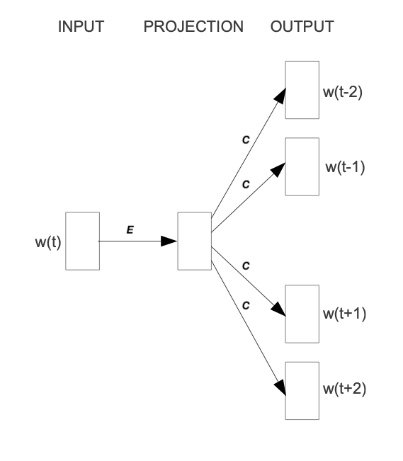
Schematic view of the Word2Vec skip-gram approach, modified. Image from [1].

To obtain an embedding for an arbitrary word, we use its one-hot representation. This vector is the input to the network, depicted on the left. In the next step, the vector is projected into its embedding representation, shown in the middle. As usual, this happens by multiplying it with a matrix, marked as E in the figure. In other words, this a forward pass in a network. The resulting (hidden) representation is optimized to predict the context words shown on the right side.

The output of the network is thus not the embedding but the context words. To predict them, we use another weight, C. When we multiply our hidden internal representation with C, we get a vector of length d, where d is our vocabulary size. This resulting vector can be interpreted as the unnormalized probability for each word to appear in the context. Thus, in training our network, we maximize the probability of actual context words and minimize the probability of non-context words. To recap, the vector flow is:

Wᵢₙₚᵤₜ × E = e | for the multiplication of the one-hot with E

out = e × C | for the multiplication of the internal representation with C

To finally obtain the embedding, we extract the internal representation. There would be more to cover here, such as the objective function (negative log-likelihood). Refer to the paper to learn more.

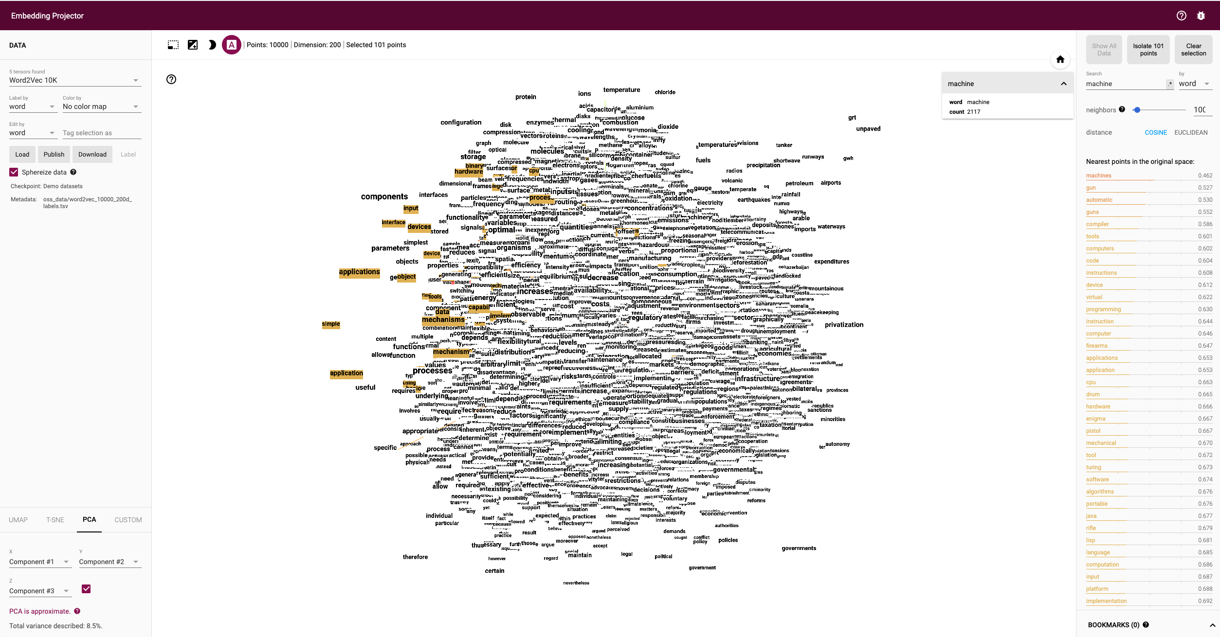
To assess the usefulness of embeddings, head over to TensorFlow’s Projector tool. It lets you explore different embeddings; in our case, the “Word2Vec 10k” dataset is suitable. Click on the “A” to enable labels. You can now visually see the similarity between related words. In the following example, I have searched for the word machine. The nearest neighbours are highlighted:

Visualization of high-dimensional embeddings. I searched for the word “*machine,” its neighbours (i.e., most similar embeddings) are highlighted. You can play around with it* *here. Image by the author.*

The Word2Vec algorithm makes two choices, as briefly mentioned above:

First, it captures local relationships. Secondly, it treats words as basic units. Other algorithms take other choices. For example, the GloVe algorithm, short for Global Vectors, creates embeddings based on global relationships and uses words as basic units. A third algorithm is FastText (see paper references here), which uses sub-word information as basic units (e.g. “this” -> “th” and “is”).

A few challenges exist, regardless of the algorithm choice: How to handle punctuation? How to handle plural words? Different word forms? Such modifications are part of the pre-processing, which often includes stemming and lemmatization. Stemming reduces a word to its stem. This technique is efficient but can create artificial word stems. Lemmatization tries to reduce a word to its base form, which is often achieved with large databases.

With the advance of modern end-to-end approaches, the importance of pre-processing has slightly become less. Only tokenization remains relevant, such as Byte-Pair encodings. Before we get there, we have to take a look at n-grams.

(Modern) n-gramns

To begin incorporating word order, we can use a so-called n-gram approach. Previously, when creating the BoW representation, we split the sentence into single words. Instead, we could also divide it into segments of two successive words, three successive words, and so on. The number of words in a row is the n in n-gram. If n is one, the parsing model is called unigram; if n is two, it is called bigram.

As an example, let’s parse “The quick brown fox jumps over the fence” with a bigram model:

[“The quick”, “quick brown”, “brown fox”, “fox jumps”, …]

As we see in this example, we slide a window over the text, with a size n and a stride of one. The stride of one causes the last word of the previous extract to be the first word of the following excerpt. Using this approach, we partially keep the relationship between words.

The representation is static. If the n parameter changes, the dataset has to be pre-processed again. Depending on the size, this can take a while. However, we can incorporate the n-gram algorithm into neural networks and let them do the “pre-processing.” This approach can be seen as modern n-grams.

From the embedding step, we use the obtained dense and informative representation vectors for every single word. To incorporate word order, we have to alter the network input slightly. Given a sentence of length l and embeddings of size e, the input is now a matrix with shape:

l x e

This matrix can be interpreted as a strange image. In image-related tasks, convolutional neural networks are highly effective, but they are not restricted to this domain. A convolution operation going over the input text-matrix can be interpreted as creating n-grams. When the kernel size is set to 2 and the stride to 1, this essentially creates a bi-gram representation. Keeping the stride but increasing the kernel’s size to 3, we obtain a tri-gram model.

The convolution operation has some beneficial properties. Among them is the location invariance. A kernel can be applied at every position of the input. If one such kernel focuses on adjective-noun combinations, it will detect them at any place. Additionally, convolution operations naturally share their weights and have significantly fewer parameters than dense layers.

The drawback of n-grams is that they only capture relationships over a limited range. For example, N-grams can not express the connection between the first and last word of a sentence. Setting the parameter n to the length of a sentence would work but would require a separate n for each differently-sized sentence. There is a better approach to handle relationships over a large span, the attention mechanism. This technique was introduced for machine translation tasks.

Machine Translation

The Machine Translation (MT) task deals with translating text from a source to a target language. For example, “Est-ce que les poissons boivent de l’eau?” (French) would be translated to “Do fishes trink water?”

Early MT research was done during the Cold War and aimed to translate Russian to English. The systems in use were mainly based on rules and required dictionaries. In the next step, the word order was corrected.

From the 1990s on, statistical MT became the focus. The core idea is to learn a probabilistic model. With an emphasis on translational tasks, this means the following: Given a sentence in a source language, we need to find the most proper sentence in the target language — i.e., the best translation.

Mathematically, this is expressed by y* = argmax_y P(y|x). The y* denotes the translation with the highest probability.

With the rules of Bayes, this description can be broken down into two separate parts: y* = argmax_y P(x|y) P(y). The first component, P(x|y), models the probability of x being the translation of y. This part is called the translational model. The second part, the language model, gives the probability of y in the target language.

In other words, the first part quantifies the probability of the source sequence, and the second part quantifies the probability of the target sequence. The translational model is learned with large text datasets in the source and target language(s).

The advance of deep neural networks also influenced the task of machine translation. Recurrent Neural Networks, RNNs, are a good choice since both the input and output are sequences. The input is the sentence to be translated; the output is the translation. Two problems emerge with a single RNN: First, the source and target sentence lengths can be different. This fact is evident in the initial example translation. The input contains eight tokens, and the output only five (depending on how you count punctuation, but the problem stays the same). Secondly, the word order can change, rendering a single one-in, one-out RNN unusable.

The solution to both problems is using two recurrent networks in a so-called Sequence-to-Sequence (Seq2Seq) layout [2,3]. The first network, named encoder, takes the input and yields an internal representation. The second network, called decoder, uses this internal representation to generate the target sequence, e.g., the translation.

A short note: The internal representation can model any knowledge about the input sentences, which includes word relationships. The problem of long-time dependencies is thus minimized.

A single RNN reads the input token-wise parsing and immediately returns a translation. In the Seq2Seq layout, the encoder reads the complete input sequence first to create an internal representation. Only then is this representation, which usually is a vector, passed to the decoder network.

This setup is trained text pairs, and the probability of the generated target sequence is seen as the loss. During training, the model, which is the combination of the encoder and decoder, maximizes the probability of appropriate translations.

This setup is all that is required to handle Seq2Seq tasks. However, as usual, one can make a couple of improvements, among them the attention mechanism.

Attention

In the vanilla sequence-to-sequence layout, the encoder compresses all information about the input sentence into a single vector. This vector is fittingly called the bottleneck layer, as it causes an information bottleneck. Despite the ability to parse endless sequences, the information from earlier steps will slowly fade as new information gets added.

The solution to this bottleneck is making all hidden encoder states accessible. In the vanilla setting, the encoder only delivers its last state, which becomes the bottleneck. This approach can be modified to save all intermediate states after the network parsed a new token. As a result, the encoder can store the per-step information and no longer compresses all knowledge into a single vector.

In the encoding step, the encoder network has access to all the per-step vectors. As a result, it can now pay attention to the most important hidden states. I’ll briefly go over the mechanism that achieves this [4].

The encoder saves all hidden states (the vectors after it parsed a new token). We then take the encoder’s current state and compute the dot-product between it and the hidden states. This operation returns a scalar number for each hidden state, which we can represent as a new vector:

[a, b, c, d, e],

where the characters represent the result of the dot product with the corresponding hidden state (e.g., a is the result of the dot product with the first hidden state). The softmax operation is then applied to this vector, yielding the attention weights. These weights express the importance of each hidden state, represented by a probability. In the last step, we multiply the hidden states with their attention score and sum the vectors up. This gives us the context vector for the current state, which is passed to the encoder (not completely right, but fine for this purpose). This process is repeated after each encoder step.

The process can be seen in this animation, taken from Google’s seq2seq repository:

Animation of the Sequence-to-Sequence process. Bold lines indicate the attention on specific encoder states. Animation from Google’s seq2seq repository.

An animation of the attention mechanism. From Google’s seq2seq.

The attention process enables the encoder to store the per-step information and lets the decoder decide which hidden states to pay attention to. These modifications have greatly improved the quality of text translation, as shown in [4].

A general drawback of recurrent networks in general, and the sequence-to-sequence approach in particular, is the low parallelizability. Recall that the output of step k+1 depends on step k; we thus have to parse all previous steps first. Therefore, we cannot run much in parallel here — except if we change the underlying network architectures. This idea leads us to Transformers.

Transformers

The Transformer [5] is a neural network architecture that utilizes the attention mechanism. Under the hood, it still uses an encoder-decoder structure but replaces the recurrent networks. Instead, the encoder is modelled by n identical layers with self-attention and regular feed-forward networks. An encoder block uses the same structure and adds another attention layer that takes the encoder’s output. The following figure, taken from [5], shows the described setup:

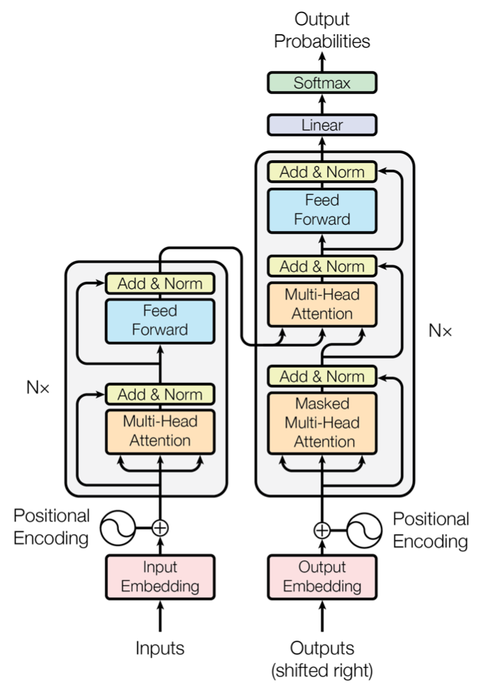
Schematic view of the Transformer architecture. On the left the encoder stack, on the right the decoder stack. Image from [5].

A second improvement is the modification of the attention procedure. In the vanilla sequence-to-sequence approach, the hidden state of the decoder calculates the dot-product with all encoder hidden states. In the improved mechanism, called Multi-Head Self-Attention, these operations are modelled as matrix multiplications.

The self-attention transforms the input to an internal representation, a weighted sum of its own timesteps. This approach can capture long-term dependencies within the sequence. The input is converted into three different representations, the Key, the Query, and the Value, to model these relationships. These representations are obtained by multiplying the input with three weights: Wₖ (for the Key), Wᵥ (Value), and Wq (Query). The computation flow is shown in the following figure [5]:

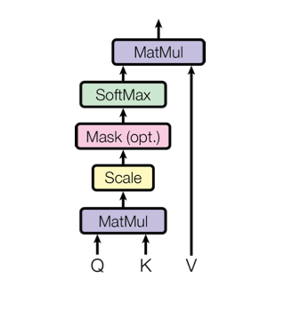
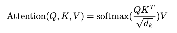
Detailed view of the attention mechanism. Q, K, and V are different representations of the same input. Image from [5].

Q and K are matrix-multiplied, scaled, optionally masked, and then softmax-ed. Finally, the result is matrix-multiplied with V. This can mathematically be expressed in the following equation:

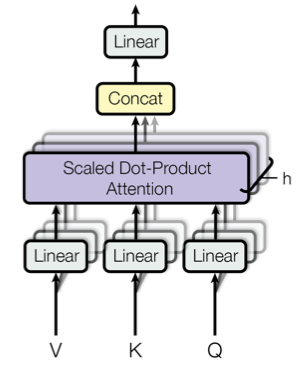
Representation of the attention mechanism as an equation. Image from [5]

Finally, there are multiple such “flows,” dubbed attention heads. Each head uses a different set of attention weights Wₖ, Wᵥ, and Wq. These weights yield multiple internal representations for the same input. The result of the individual attention heads are then concatenated, as shown in the following figure [5]:

Schematic visualization of the Multi-Head Attention mechanism. The individual vectors are concatenated before being fed into a linear layer. Image from [5].

These computations are done in the encoder and decoder blocks and can be run in parallel. This parallelization is one of the reasons why the Transformer approach is faster than vanilla RNN models. Further, the Transformer uses Byte Pair encoding, enabling him to generalize to unseen words. Rare words are a common problem, as are languages with compounding. Think of Germany’s crazy nouns such as “Baumhausprüfgesellschaft” (“Society that checks treehouses”). I highly doubt that such combinations are present in typical training data. So the idea is to use sub-word tokens, the aforementioned Byte Pair encoding: We extract the most frequent sub-words from the training data, such as “th” and “ng.” With such a vocabulary, we can then model an (unknown) word as a combination of the Byte Pairs.

To model word relationships, we have to preserve the information about the input order. The simple idea is to modify the tokens’ embedding vectors. We add a signal to each embedding that models the distance between vectors, the step-wise information.

More details could be covered here, but this will lead away from this post’s theme. If you are interested, I recommend Jay Alammar’s description, “The Illustrated Transformer.”

After the progress covered so far, one might get the impression that natural language can now be parsed fairly easily. This is not the case. A couple of problems persist. Coming back to word embeddings, we can now use the attention mechanism to model word relationships. However, consider the sentence “He opened a bank.” From the context, it becomes clear that the “bank” is the financial institution. Now consider “She sat on the bank.” Again, the context information explains that the “bank” is the thing used to sit on.

Word2Vec or similar frameworks only create one vector per token. However, as we have noticed, the meaning of a word is determined by its context. And the frequent context might vary between the training data (used to obtain the embeddings) and the test data. So how can we solve this? By using transfer learning.

Transfer Learning, Language Models and ELMo

In computer vision tasks, transfer learning is a standard procedure. First, learn a model on task A, then use the weights for B. Usually, tasks A and B have been trained on the same data types. Further, the problems being solved (object detection, classification, translation) are sufficiently similar. This concept can be expanded to the NLP domain.

We pretrain a model on an extensive dataset, modify the model, and reuse it for our task. In the pretraining step, the model has already learned linguistic features, such as syntax or semantics. The advantage is the decreased need for data for the new task.

A standard pretraining task is language modelling. When we train a language model, we predict the upcoming word based on the previous ones. For this task, ELMo [6] becomes relevant. ELMo, short for Embeddings from Language Models, consists of LSTM layers. Several of these layers are stacked and trained to predict the upcoming word. Additionally, the model goes one step further: it is a bi-directional language model. The sequences are parsed in both directions. To obtain an embedding vector, we concatenate the hidden layers and sum them up (simplified), as shown in this figure, taken from Jay Alammar’s introduction to BERT and co.:

Schematic representation of the ELMo process to compute embeddings. Image from Jay Alammar’s introduction to BERT and co.

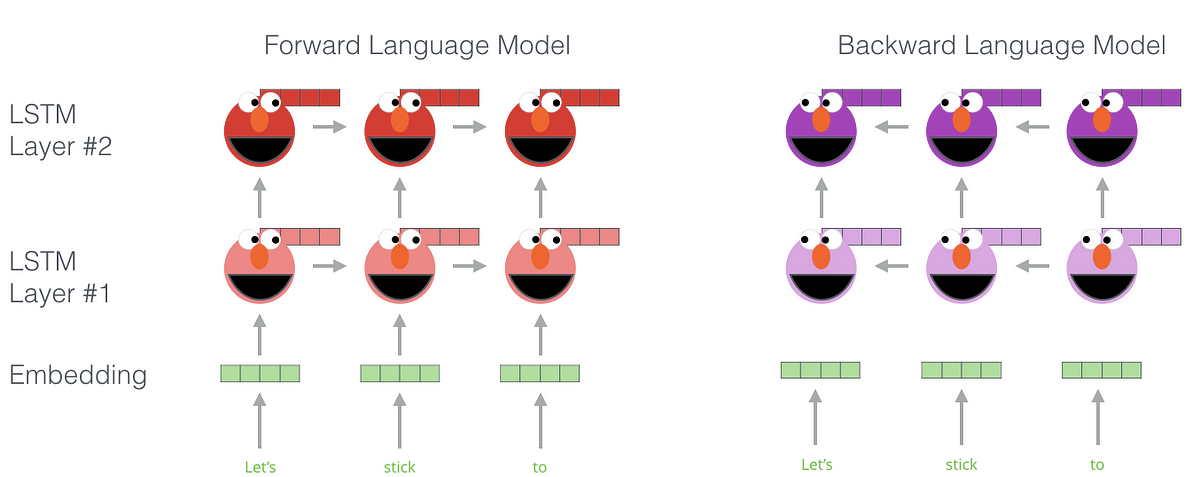
Once we have a fully-trained model, we can obtain our embeddings by querying the model with our sentences. How does this help us get context? ELMo has been trained on many data, where it had to predict the next word. And this task required it to learn context. For example, “He sat on the [bank]” and “He went to the [bank]” both end with “bank,” and the model has to learn different meanings of the same word.

The vectors one obtains from such a model incorporate this context information — they are contextualized embeddings. Thus, we get two different vectors for the previous “bank” example, depending on the context of “bank.” The embeddings are then used in our main task; the ELMo model serves as a feature extractor. But it is slow; we cannot do a table lookup but have to load the (potentially huge) model. And it relies on recurrent networks. This leads to BERT.

BERT

What has worked when going from the vanilla, RNN-based sequence-to-sequence approach also works for the ELMo model. We can replace the LSTM layers with a stack of Encoder blocks, which we know from the Transformer. These modifications give us the BERT [7] model, short for Bi-directional Encoding Representation from Transformers. Parts of the input sequence are masked, which makes this a masked language model. We achieve bi-directionality by randomly masking tokens (default: 15 %); we do not need to parse the sequence in both directions.

The output of BERT is a layer of dimension hidden_size, set to 768 in the base model (12 Encoder blocks stacked). These output vectors are our embeddings, and they are again contextualized. As with ELMo’s embeddings, we can take them and utilize them for our specific task. Or we can just use BERT; it’s highly effective on a wide range of tasks. We can use it for sentiment analysis, question answering, named entity recognition (tagging tokens as, e.g., nouns). With 110 million parameters in the base and 340 million in the large variant, there are a couple of things you can do. But we are not at a billion yet. Enter GPT-2.

GPT-2

The idea behind GPT-2 [8] is close to that of BERT: Train one large language model on a massive text corpus. GPT is short for Generative Pre-Training, and the 2 indicates that this is the second iteration. The first iteration was called OpenAI Transformer [9] and stacked Transformer Decoder layer. BERT later succeeded this architecture. Coming back to GPT-2, the model has between 117 million and 1542 million parameters — 1.5 trillion parameters. As it is a language model, each task it can perform is modelled as a completion task. Let’s say you want to translate from English to Latin. First, the model is trained as a translational system, and during inference time, you give it a prompt like

“The government has issued the newest round of scholarships.=”

The “=” indicates that the model has to complete (i.e., translate) the sentence. During training, it saw pairs of “<English>=<Latin>” and thus learned the properties of the “=” prompt. The translational task is not the only one; GPT -2 also excels at summarization and question answering.

Different from the BERT model, GPT-2 is not fine-tuned on the target task. After BERT was trained on the base text corpus, it was fine-tuned for the individual problems. This step is obsolete for GPT-2, making it a zero-shot setting. In other words, it is a general model capable of performing a wide range of tasks not directly trained for. In addition, its ability to generate coherent text, often on par with human work, lead to ethical consideration. With access to a large GPT-2 model, one can, for example, generate fake news, impersonate others, or produce massive amounts of high-quality spam.

Therefore, OpenAI, the organization behind the GPT networks, initially decided not to release the entire model. Instead, only trained weights for the 117 and 345 million parameter models were published. However, at the end of 2019, the researchers also made the large models available, giving anybody versed enough access to a 1.5 billion parameter model.

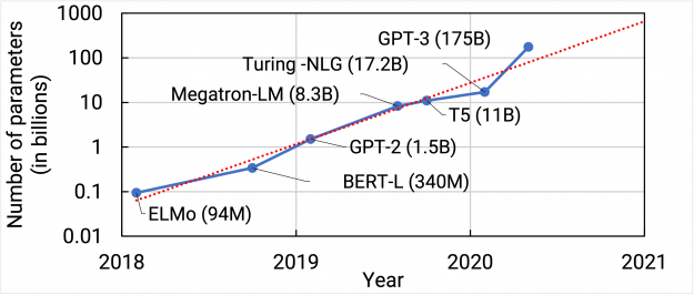
Even though we have now reached more than one billion parameters, there are still larger models. There are several architectures in the range of billion parameters, and two with trillion+ parameters.

Switch Transformer

There are several architectures with billion parameters. The following figure, taken from Nvidia’s blog, shows the growth of language models:

Since we have reached the billion parameter threshold already, I will introduce a trillion parameter model, the Switch Transformer [10]. The key change that this architecture uses is the Mixture of Experts (MoE) approach. Usually, the models use the same parameters for all inputs. Whether the input is an image of a cat or a dog, the used weights are the same. In the MoE setting, the model selects different parameters (think routes) for each input. This approach corresponds to sparse neural networks, where only a subset of the weights is used simultaneously. The following figure makes this clear (taken from [10]):

The figure shows a modified transformer encoder block, as introduced previously. In this original block, the flow of the information is predefined by the block’s layout. In contrast, the Switch Transformer block maintains several feed-forward neural networks (as opposed to a single one). A router layer then selects which of these networks, called Experts, the current input is forwarded toward. This approach efficiently maximizes the parameter count of a Transformer. And because only one Expert is consulted, it is still computationally feasible.

There are a couple of other tricks that enable that many parameters. Among them are parallelization strategies. In data-only parallelism, the workers work on independent data splits, and each worker uses the same weights. In model parallelism, the model’s layers are divided across the workers. This strategy is helpful once the activations grow too large to fit on a single device. The Switch Transformer combines both techniques. There are many more details in use. However, covering them exceeds this post’s scope, so I encourage you to do your own study. I especially recommend the discussion and the future research direction sections.

—

With the Switch Transformer having more than a trillion parameters, we have reached the end of our journey. But it’s certainly not that all NLP problems are solved. For example, current research focuses on making large models smaller (distillation) and mitigating bias. There is much that we can expect from upcoming publications.

—

Summary

Natural Language Processing has seen tremendous development. Starting from one-hot vectors to represent tokens, it has advanced to embeddings to capture meaning more precisely. Slowly, these vectors were no longer obtained from Word2Vec or similar frameworks but extracted from language models (ELMo, BERT). These models started with 100 to 300 million parameters. Quickly, it became apparent that more parameters achieve better scores, so research continuously scaled the number of weights. The GPT-2 model then broke the billion parameter threshold and was superseded by even larger models. Training this many parameters is challenging and would not have been possible without massively increased compute. Powered by TPUs, the Switch Transformer then reached more than a trillion parameters. And that’s only the beginning.

References

[1] Mikolov et al., Exploiting Similarities among Languages for Machine Translation, 2013, arXiv
[2] Sutskever et al., Sequence to Sequence Learning with Neural Networks, 2014, Advances in neural information processing systems (NIPS)
[3] Cho et al., Learning phrase representations using RNN encoder-decoder for statistical machine translation, 2014, arXiv
[4] Bahdanau et al., Neural Machine Translation by jointly learning to align and translate, 2015, ICLR
[5] Vaswani et al., Attention Is All You Need, 2017, NIPS
[6] Peters et al., Deep contextualized word representations, 2018, arXiv (slides)
[7] Devlin et al., BERT: Pretraining of Deep Bidirectional Transformers for Language Understanding, 2018, arXiv (slides)
[8] Radford et al., Language Models are Unsupervised Multitask Learners, 2019, OpenAI blog
[9] Radford et al., Improving Language Understanding by Generative Pre-Training, 2018, OpenAI blog
[10] Fedus et al., Switch transformers: Scaling to trillion parameter models with simple and efficient sparsity, 2021, arXiv