Visualizing Image Augmentation Pipelines with Streamlit

Across all data domains, images have received the greatest amount of attention. Just consider convolutional neural networks: their kernels lend themselves easily to detecting objects in images, regardless of their position. Or, the mighty ImageNet dataset. This million-samples collection had and still has a tremendous impact on the evolution of new network architectures. The sheer amount of samples has led researchers and practitioners (like you and me) to become creative and develop novel solutions. But what if you do not have the resources — time, money, manpower — to work with a dataset that large? Augmentations are the solutions, and that is what we’ll focus on now.
In short, augmentations are simply transformations of the data to improve a machine learning solution’s performance. For example, if we turn an image upside down, we have applied a transformation (horizontal flipping); that is, we have augmented the image. Besides common augmentations such as flipping or rotating a data sample, there are more advanced methods available, including blurring images or making them noisier. What lies behind these transformations is everybody’s favorite: mathematics.
Before you now frantically search for underlying math, rest assured that solutions are already available. The two major machine learning frameworks, PyTorch and TensorFlow, both provide libraries that do the job. Besides these framework-specific solutions, there are framework-agnostic (python) libraries available. The Albumentations package is one of them. This free and open-source package provides plenty of operations to apply.
Often, we are interested in what the transformations do to our images. That is where Streamlit, a great tool for quickly developing data applications, comes into play. In a mere few hours, we can create a neat application that lets us visualize the effect of the augmentations on our own image data.
If you are interested in the code for such an application, then jump directly to this post’s GitHub repository. You can also try it live here. With this being said, let’s quickly walk through this albumentations demo.
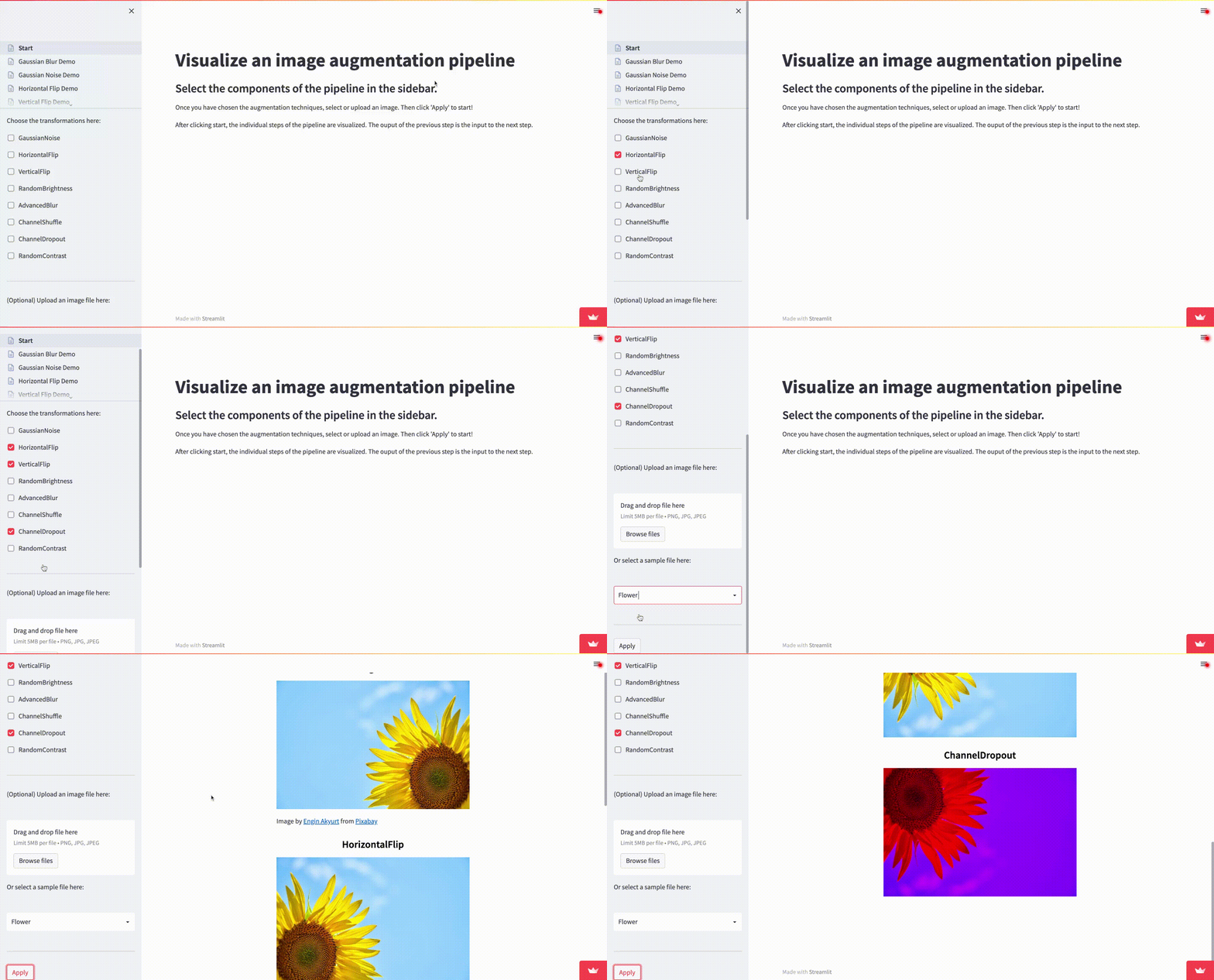
On the start page, you can assemble your preprocessing pipeline by selecting the augmentations on the left. After clicking ‘Apply’, an image of your choice will be pushed through the pipeline. After each transformation, the sample’s current state is visualized in the center of the screen. In this view, the output of step n is the input to step n+1; that is, the already transformed image is augmented further. You can see this in the gif below or explore it for yourself here. The dog image used in the demonstration is by Marsha Jones from pixabay. Readers following me for a long time might notice the similarity to an earlier project I did: visualizing audio transformations.

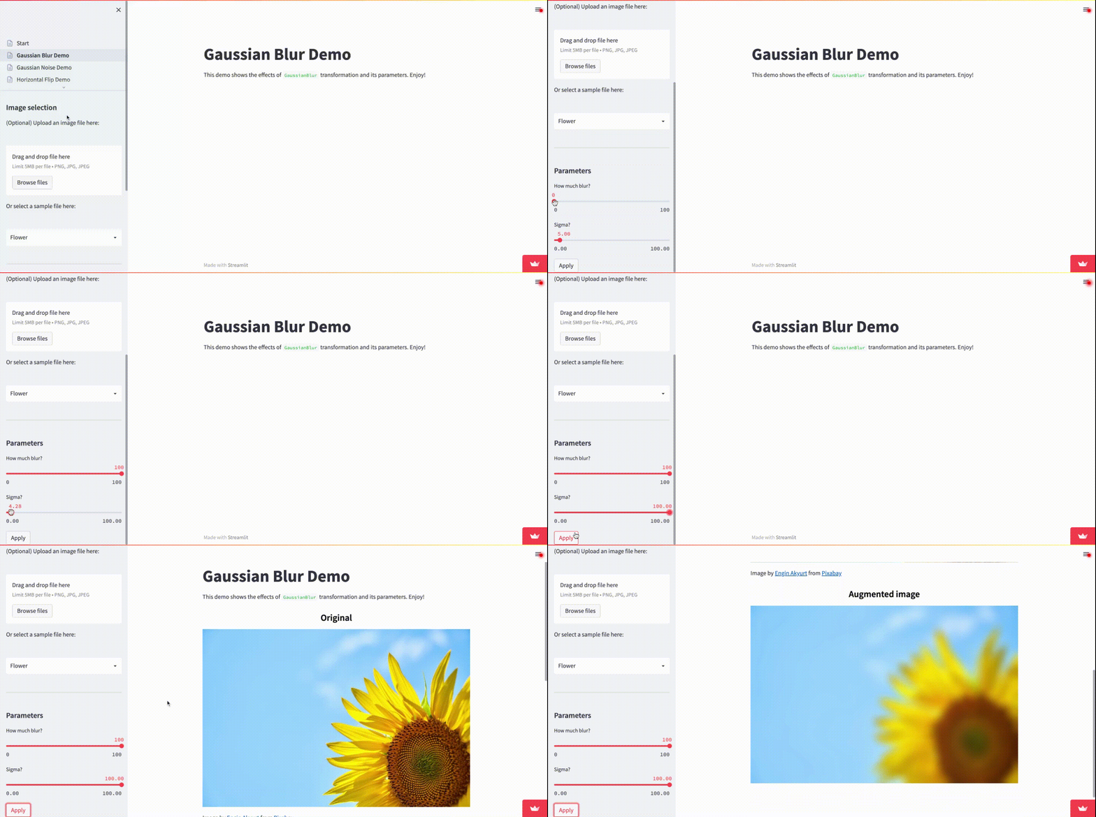
If you want to explore individual augmentations in detail, then select one of the subpages. On each of them, a specific augmentation and its parameters can be selected and their effects visualized. For example, for the blurring operation, we can select the blurring limit (the blurring kernel’s size) and the sigma limit (the kernel’s maximum standard deviation). By changing the sliders and applying the parameters, we see their effects on the main screen, as shown below.

This little application helped me better understand and build image augmentation pipelines. Currently, only the most frequent transformations are included; leave a reply on the GitHub repository if you want others to be included, too!
